Las hojas de cálculo ofrecen potentes capacidades de análisis, pero a veces parece que les falta esa capa adicional de información. Cuando hay una cantidad enorme de datos, es difícil resumir o sacar conclusiones desde una vista básica de hoja de cálculo.
That's where pivot tables come in. Most Excel power users use pivot tables as their bread and butter. But you can also use pivot tables in Google Sheets.
Here, I'll walk you through how to create and use pivot tables in Google Sheets.
Tabla de contenido:
¿Estás debatiendo entre Microsoft Excel y Google Sheets? Consulta nuestro análisis de aplicaciones para descubrir cuál es la adecuada para ti: Google Sheets frente a Excel.
¿Qué es una tabla dinámica en Hojas de cálculo de Google?
A pivot table in Google Sheets is a built-in spreadsheet tool that lets you reorganize, summarize, and analyze large datasets based on whatever dimensions you choose.
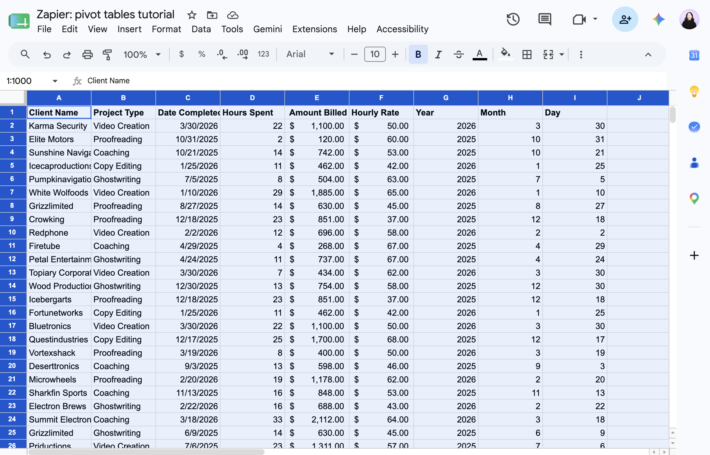
Think of it this way. Normal spreadsheets typically have "flat data" represented by two axes: horizontal (columns) and vertical (rows). For example, a sales team might track their sales in individual rows, with each column offering different information about that sale. A pivot table shifts (or pivots) those axes to introduce a third dimension. So instead of looking at individual sales, you can see aggregated data like how many units each sales rep sold per product.
While you could pull many of these insights using formulas, the pivot table allows you to distill it in a fraction of the time and with less chance for human error.
How to create a pivot table in Google Sheets using Gemini
The mechanics of creating a pivot table in Google Sheets are pretty straightforward. Knowing which elements to plug in where—so your pivot table actually surfaces the information you care about—is a different story.
If you want to save yourself the headache, just tell Gemini what you want to know, and it'll build the pivot table for you.
Here's what Gemini created when I asked it to create a pivot table and tell me how much we billed in 2025 for each client across different project types. (It's one sentence versus the multiple steps I'm about to walk you through for the same results.) Gemini even automatically generated a summary of how the data was used to build the pivot table.

How to create a pivot table in Google Sheets manually
If you're more of a DIY-er, respect—I admire the commitment and wish I had it. Here's how to create a Google Sheets pivot table step by step.
As a reminder, this is the question we're asking: How much did we bill in 2025 for each client across different project types? To follow along, grab our demo spreadsheet.
Select the dataset, including the column headers, that you want to summarize or analyze. If your data set contains columns without headers, you'll need to name these columns in order to create a pivot table.
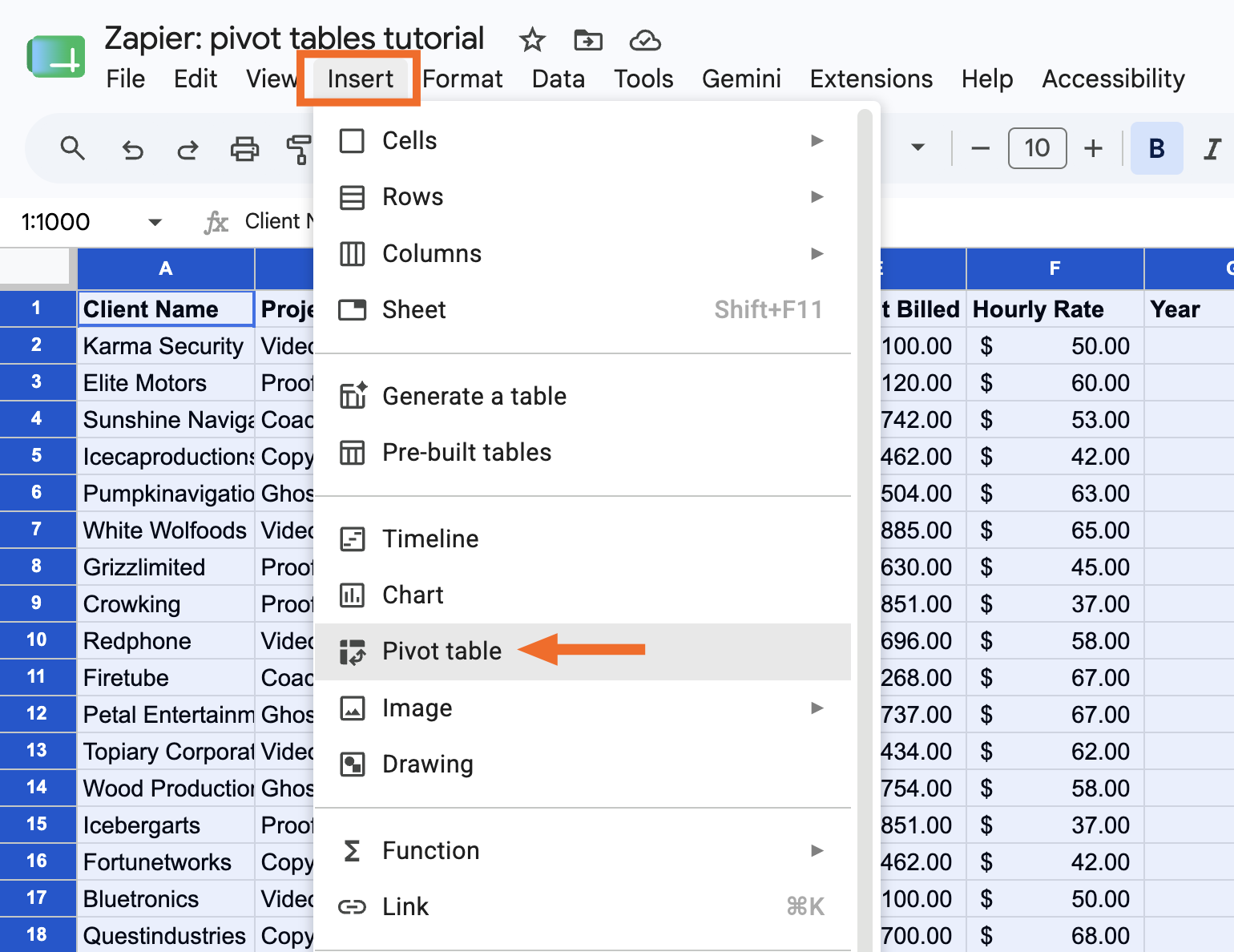
Haga clic en Insertar y seleccione Tabla dinámica.
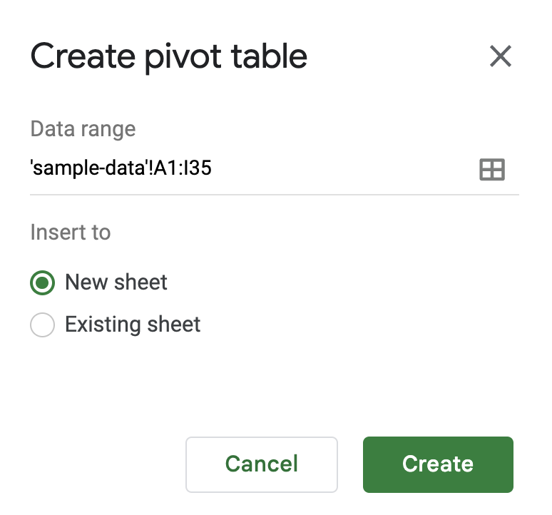
In the Create pivot table panel that appears, choose if you want to insert your pivot table into a new sheet or an existing sheet. Then click Create.
In the Pivot table editor panel that appears, you'll see a few elements you can add to configure your pivot table.
Rows: Choose which field you want to list down the left side of your pivot table. Google Sheets will pull every unique value from that field and stack them as rows. In our example, that's Client Name, so each client gets its own row.
Columns: Choose which field you want to spread across the top of your table. Each unique value will become its own column header. In our example, that's Project Type, so each project type gets its own column.
Values: Choose what number you want to see where each row and column meet. You can show these values in different ways (sum, average, count) depending on the value type. In our example, we want the SUM of Amount Billed, so each cell shows the total billed for that client and project type.
Filters: Choose a field to limit which data gets included in your table at all. In our example, we filter by Year and select only 2025.


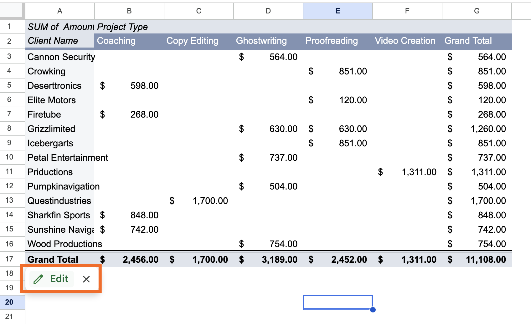
That's it! Now you have a pivot table that answers the question, "How much did we bill in 2025 for each client across different project types?"
Cómo actualizar una tabla dinámica en Hojas de cálculo de Google
Let's say you've edited your original source data. These changes should automatically be reflected in your pivot table. If you don't see the changes reflected, refresh your web page. It may take a minute depending on the volume of data.
If you've added new rows or columns of data to your original source data, however, a simple refresh won't do the trick. Instead, you need to update your pivot table's data range to include the new rows or columns.
Coloque el cursor sobre la tabla dinámica y haga clic en Editar.
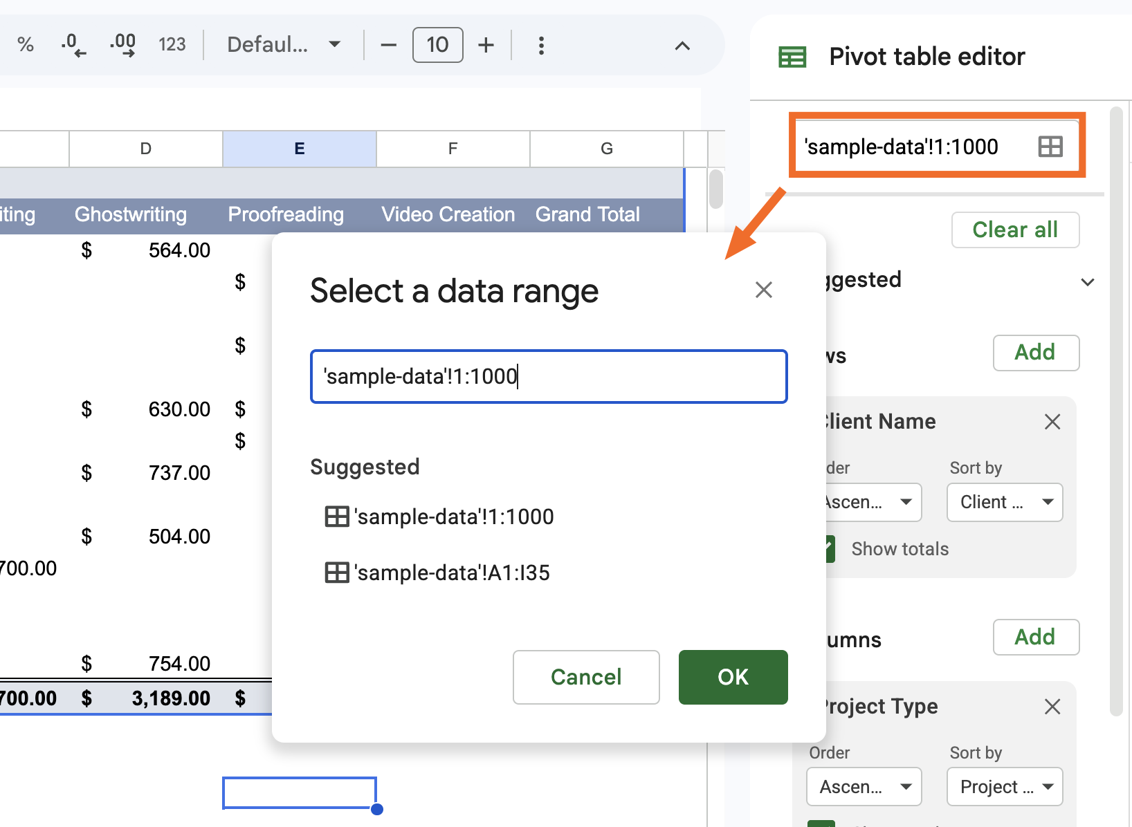
Click the Select data range icon at the top of the panel, and enter your new data range.


Cómo crear y usar tablas dinámicas en Hojas de cálculo de Google: Preguntas frecuentes
¿Aún tienes preguntas sobre cómo usar tablas dinámicas en Hojas de cálculo de Google? Consulta las respuestas a estas preguntas frecuentes para que puedas aprovechar al máximo tus hojas de cálculo.
¿Las tablas dinámicas se actualizan automáticamente en Hojas de cálculo de Google?
Yes, with one caveat. If you edit existing cells within your data range, changes will automatically show up in your pivot table. If you add new rows or columns outside of it, you'll need to manually update the data range first.
¿Puede una tabla dinámica extraer información de varias hojas de cálculo?
Las tablas dinámicas en Hojas de cálculo de Google solo pueden hacer referencia a una única hoja de cálculo. Si desea que su tabla dinámica haga referencia a datos de varias hojas de cálculo, primero deberá combinar esos datos en una sola hoja de cálculo. Luego, puedes crear una tabla dinámica como lo harías normalmente.
¿Es posible tener dos tablas dinámicas en una hoja?
Puede insertar varias tablas dinámicas en una hoja de cálculo de Google Sheets.
Crea una tabla dinámica como lo harías normalmente.
En el panel Crear tabla dinámica que aparece, seleccione Hoja existente e ingrese la hoja de cálculo y la celda donde desea agregar su nueva tabla dinámica.
Haga clic en Crear.
¿Es posible fusionar dos tablas dinámicas?
No es posible fusionar dos tablas dinámicas en Hojas de cálculo de Google, pero existe una solución alternativa. Combine los datos de origen originales de ambas tablas dinámicas en una hoja de cálculo y luego cree una nueva tabla dinámica.
Automatizar Hojas de cálculo de Google con Zapier
Pivot tables are only as good as the data behind them. Zapier connects Google Sheets to 9,000+ apps, so you can automatically pull in data from wherever you need it, including form submissions, CRM updates, and ad leads.
And if you're already working in Claude, ChatGPT, or another AI tool, Zapier MCP lets you go further: you can ask your AI assistant to pull data from your connected apps, update your spreadsheet, or practically anything else you can think of, all without leaving your chat window. You could even ask it to figure out which client you billed the most in 2025, pull up their contract in Docusign, and draft a renewal email. Discover more ways to automate Google Sheets.
Lectura relacionada:
Cómo agregar un menú desplegable en Hojas de cálculo de Google
Plantillas gratuitas de Hojas de cálculo de Google para aumentar la productividad
Cómo usar IMPORTRANGE en Google Sheets: Una guía paso a paso
This article was originally published in September 2018 by John Thomas. The most recent update was in June 2026.